library(tidyverse)
library(vegan)

neon <- read_csv("~/Bio 478 Lab/NEON_soilMAGs_soilChem.csv") |>
filter(!is.na(phylum))Lab 13: Soil MAG Community Analysis from NEON Sites
Data Preparation
This dataset contains MAGs collected from NEON soil metagenomes.
Taxonomy and sample site IDs are used to evaluate microbial community structure.
Distribution of MAGs Across Sites
Counting MAGs per site illustrates sampling depth differences and general variation in recovered genome counts.
neon |>
  count(site_ID, name = "n_MAGs") |>
  arrange(desc(n_MAGs)) |>
  slice_head(n = 15) |>
  ggplot(aes(x = reorder(site_ID, n_MAGs), y = n_MAGs)) +
  geom_col() +
  coord_flip() +
  xlab("Site") +
  ylab("MAG Count") +
  ggtitle("Top Sites by Number of MAGs")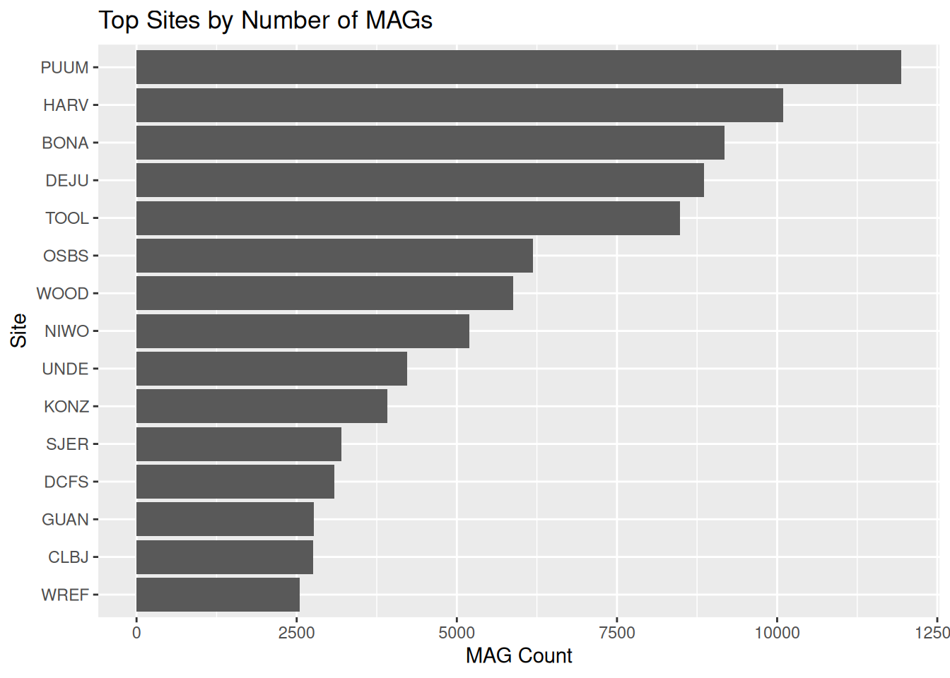
Dominant Phyla Across All Sites
Phylum frequency highlights which broad microbial lineages are most detected in the MAG dataset.
neon |>
  count(phylum, name = "n_MAGs") |>
  arrange(desc(n_MAGs)) |>
  slice_head(n = 15) |>
  ggplot(aes(x = reorder(phylum, n_MAGs), y = n_MAGs)) +
  geom_col() +
  coord_flip() +
  xlab("Phylum") +
  ylab("MAG Count") +
  ggtitle("Most Represented Phyla")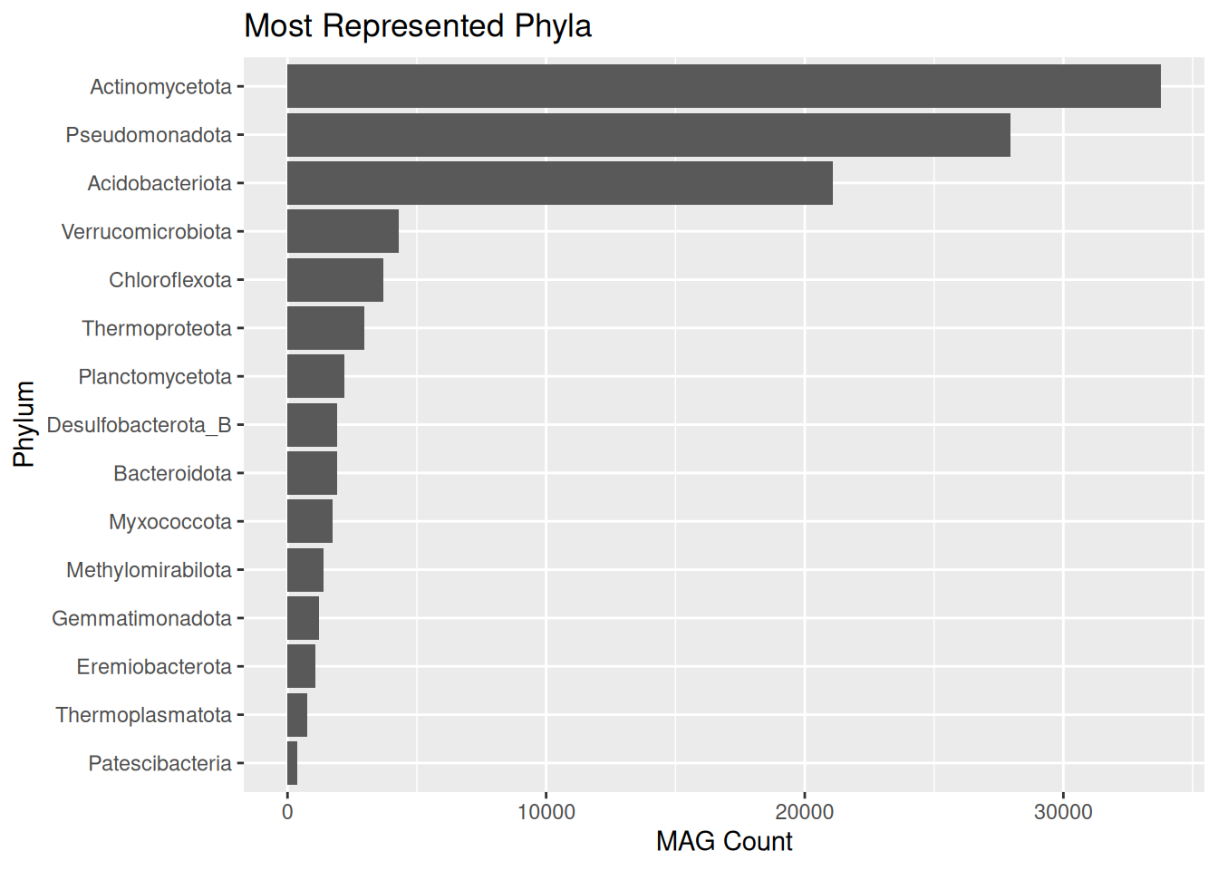
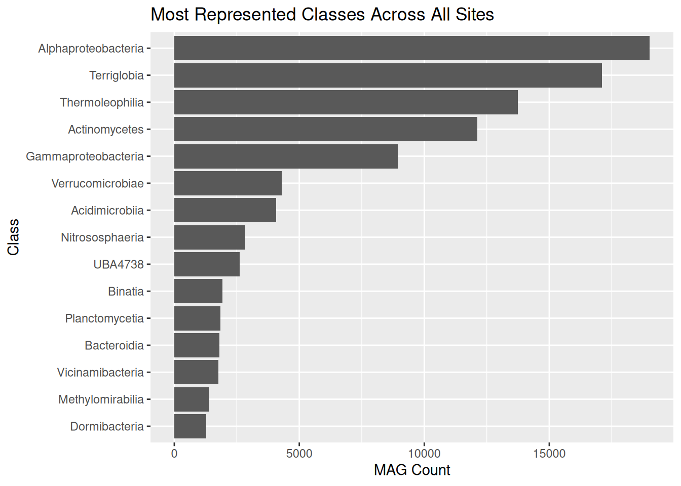
Dominant Classes Across All Sites
Class-level patterns refine broad phylum profiles and show more detailed taxonomy differences.
if ("class" %in% names(neon)) {
  neon |>
    filter(!is.na(class)) |>
    count(class, name = "n_MAGs") |>
    arrange(desc(n_MAGs)) |>
    slice_head(n = 15) |>
    ggplot(aes(x = reorder(class, n_MAGs), y = n_MAGs)) +
    geom_col() +
    coord_flip() +
    xlab("Class") +
    ylab("MAG Count") +
    ggtitle("Most Represented Classes Across All Sites")
}
Phylum Composition by Site
Relative phylum proportions show taxonomic differences among sampling locations.
MAG count per phylum serves as a proxy for presence because read abundance data are not included in this dataset.
phylum_rel2 |>
  ggplot(aes(x = site_ID, y = rel_abundance, fill = phylum_top)) +
  geom_col() +
  xlab("Site") +
  ylab("Relative Abundance") +
  ggtitle("Relative Phylum Proportions at Each Site") +
  scale_y_continuous(labels = scales::percent_format(accuracy = 1)) +
  theme(axis.text.x = element_text(angle = 60, hjust = 1))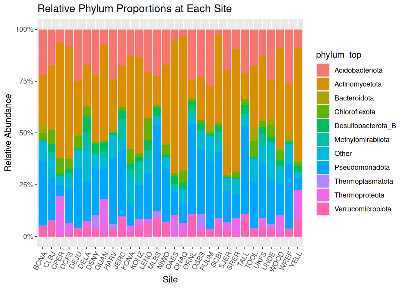
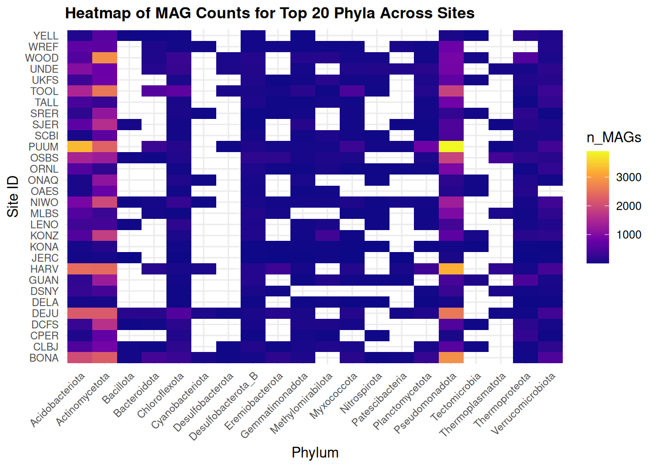
Heatmap of Phylum Counts by Site
This heatmap visualizes absolute phylum-level presence by site.
top20 <- neon |>
  count(phylum) |>
  arrange(desc(n)) |>
  slice_head(n = 20) |>
  pull(phylum)

heat_df <- neon |>
  filter(phylum %in% top20) |>
  count(site_ID, phylum, name = "n_MAGs")

ggplot(heat_df, aes(x = phylum,
                    y = site_ID,
                    fill = n_MAGs)) +
  geom_tile() +
  scale_fill_viridis_c(
    option = "C",
    direction = 1,
    na.value = "white"
  ) +
  xlab("Phylum") +
  ylab("Site ID") +
  ggtitle("Heatmap of MAG Counts for Top 20 Phyla Across Sites") +
  theme_minimal() +
  theme(
    axis.text.x = element_text(
      angle = 45,
      hjust = 1,
      size = 8
    ),
    axis.text.y = element_text(size = 8),
    plot.title = element_text(size = 12, face = "bold")
  )
Alpha Diversity of MAG Communities
Alpha diversity describes within-site diversity.
Richness counts detected phyla, while the Shannon index increases as both richness and evenness rise.
alpha_long |>
  ggplot(aes(x = reorder(site_ID, Value), y = Value)) +
  geom_col() +
  facet_wrap(~ Metric, scales = "free_y") +
  xlab("Site") +
  ylab("Diversity Value") +
  ggtitle("Alpha Diversity (Shannon Index and Richness)") +
  theme(axis.text.x = element_text(angle = 60, hjust = 1))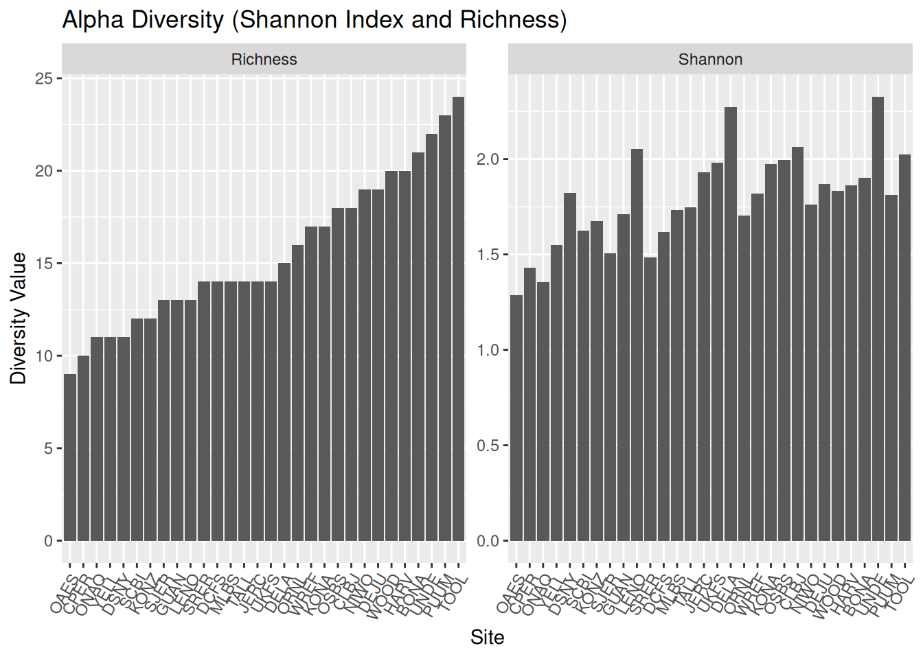
Shannon Diversity vs Soil pH
Shannon diversity is compared to soil pH to examine possible environmental influence.
ggplot(alpha_env, aes(x = soil_pH, y = Shannon)) +
  geom_point(size = 3, alpha = 0.7) +
  geom_smooth(method = "lm", se = FALSE) +
  xlab("Soil pH") +
  ylab("Shannon Diversity") +
  ggtitle("Relationship Between Shannon Diversity and Soil pH")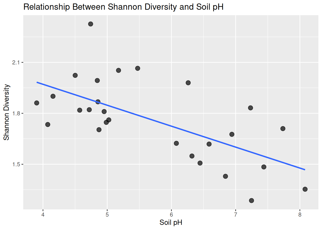
Richness vs Soil Moisture
Richness is plotted against soil moisture to explore another environmental gradient.
ggplot(alpha_env, aes(x = moisture, y = Richness)) +
  geom_point(size = 3, alpha = 0.7) +
  geom_smooth(method = "lm", se = FALSE) +
  xlab("Soil Moisture") +
  ylab("Richness") +
  ggtitle("Richness Across Soil Moisture Gradient")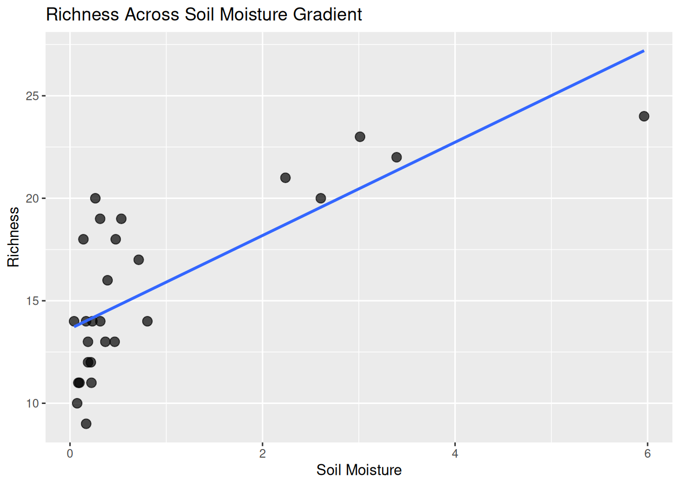
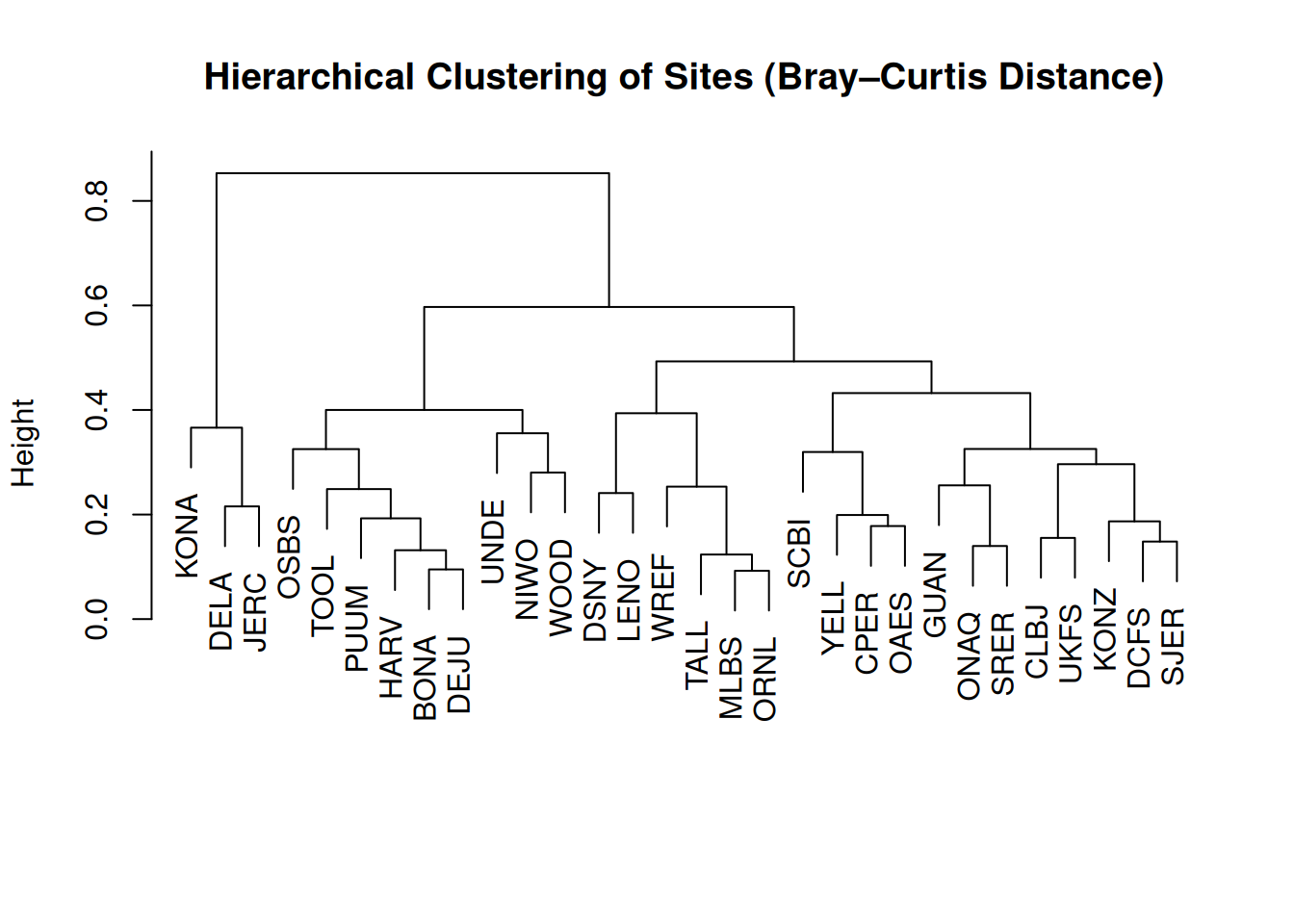
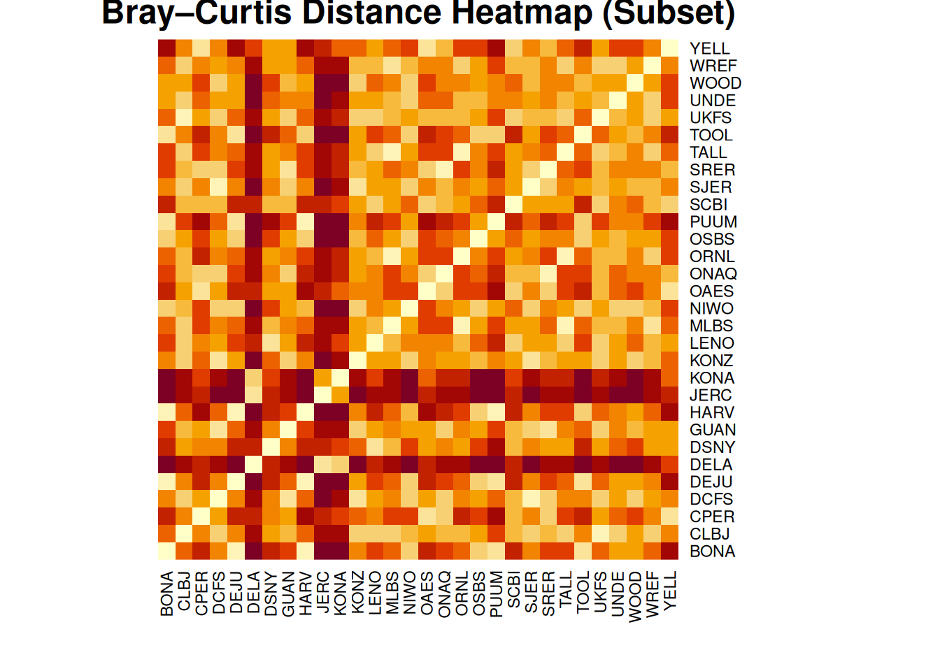
Bray–Curtis Distance Between Sites
Bray–Curtis measures compositional dissimilarity (0 = identical, 1 = no shared taxa).
Site clustering and heatmaps reveal similarities in microbial structure.
plot(
  hclust(bray_dist, method = "average"),
  labels = comm_matrix$site_ID,
  main = "Hierarchical Clustering of Sites (Bray–Curtis Distance)",
  xlab = "", sub = ""
)
n_show <- min(30, nrow(comm_only))
bray_mat <- as.matrix(bray_dist)[1:n_show, 1:n_show]
rownames(bray_mat) <- comm_matrix$site_ID[1:n_show]
colnames(bray_mat) <- comm_matrix$site_ID[1:n_show]

heatmap(
  bray_mat,
  Rowv = NA, Colv = NA,
  scale = "none",
  main = "Bray–Curtis Distance Heatmap (Subset)"
)
PCA Ordination Based on Phylum Counts
PCA provides a linear ordination alternative to NMDS.
ggplot(pca_df, aes(x = PC1, y = PC2)) +
  geom_point(size = 3, alpha = 0.7) +
  xlab(paste0("PC1 (", pc1_var, "%)")) +
  ylab(paste0("PC2 (", pc2_var, "%)")) +
  ggtitle("PCA of Sites Using Phylum Counts") +
  theme_minimal()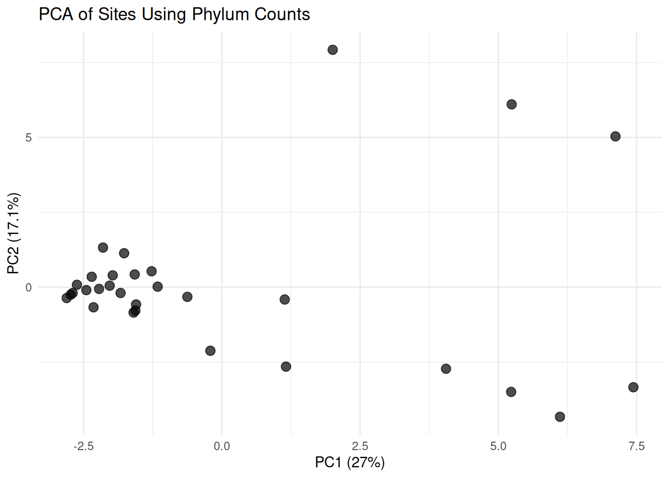
NMDS Ordination of Sites
NMDS projects multidimensional distance data into two axes.
Samples positioned closely contain more similar MAG composition.
ggplot(ord_df, aes(x = MDS1, y = MDS2)) +
  geom_point(size = 3, alpha = 0.7) +
  xlab("NMDS1") +
  ylab("NMDS2") +
  ggtitle("NMDS Ordination of Sites (Bray–Curtis)") +
  theme_minimal()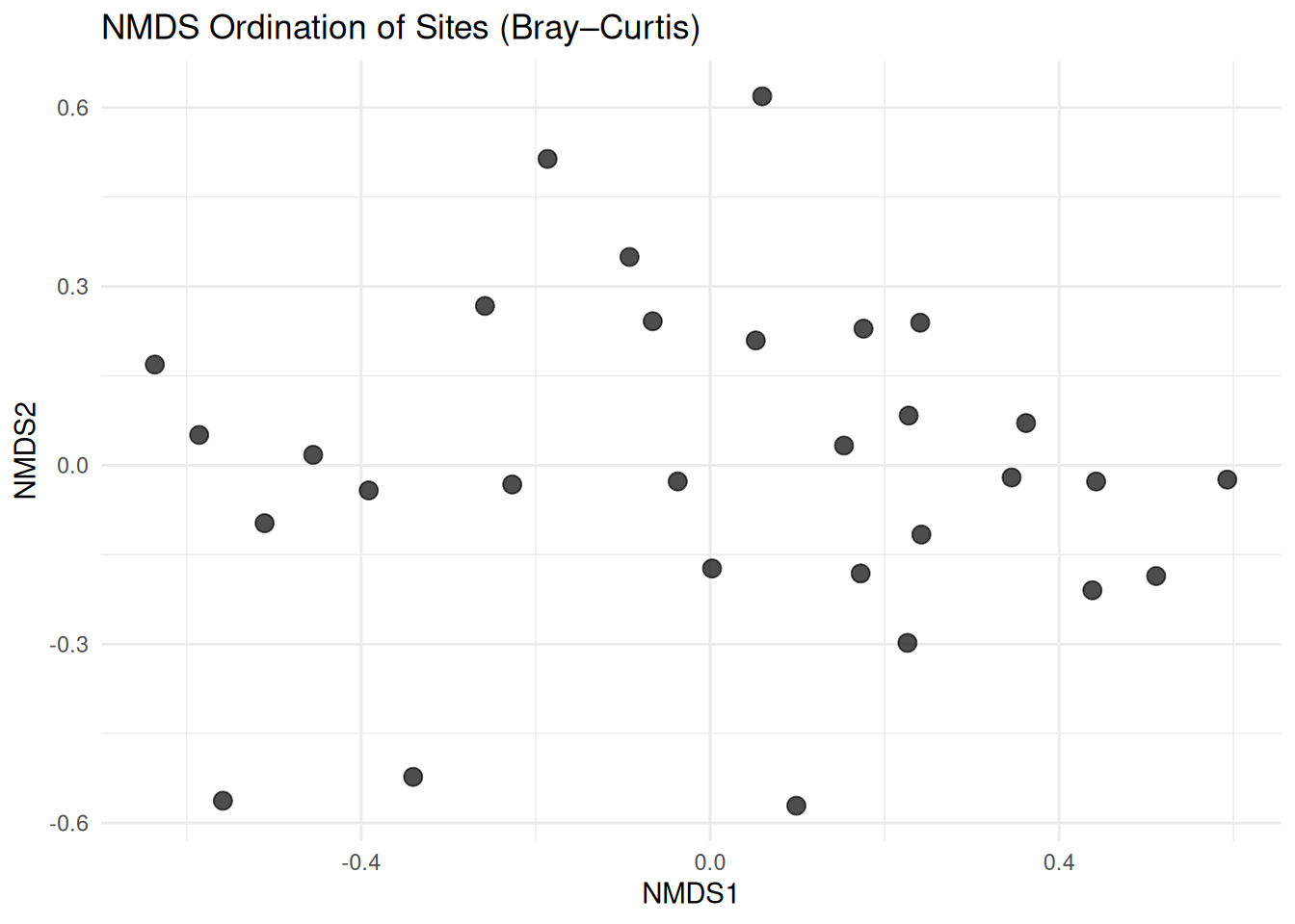
NMDS Ordination Colored by Soil pH
Overlaying soil pH reveals whether environmental gradients align with compositional differences in ordination space.
ggplot(ord_env, aes(x = MDS1, y = MDS2, colour = soilInWaterpH)) +
  geom_point(size = 3) +
  scale_colour_viridis_c(option = "C", na.value = "grey70") +
  xlab("NMDS1") +
  ylab("NMDS2") +
  ggtitle("NMDS Ordination with Soil pH Gradient") +
  theme_minimal()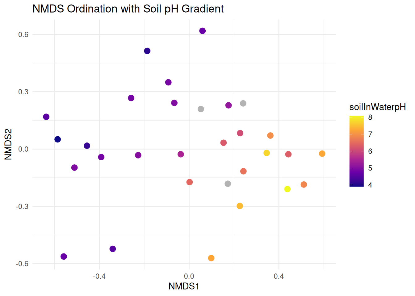
NMDS with Convex Hull By Site
Convex hull polygons outline clusters of points for each site in ordination space.
hull_df <- ord_df |>
  group_by(site_ID) |>
slice(chull(MDS1, MDS2))ggplot(ord_df, aes(MDS1, MDS2, colour = site_ID)) +
geom_point(size = 3, alpha = 0.7) +
geom_polygon(
data = hull_df,
aes(fill = site_ID),
alpha = 0.12,
colour = NA
) +
guides(fill = FALSE) +
xlab("NMDS1") +
ylab("NMDS2") +
ggtitle("NMDS with Site Convex Hull Groups") +
theme_minimal()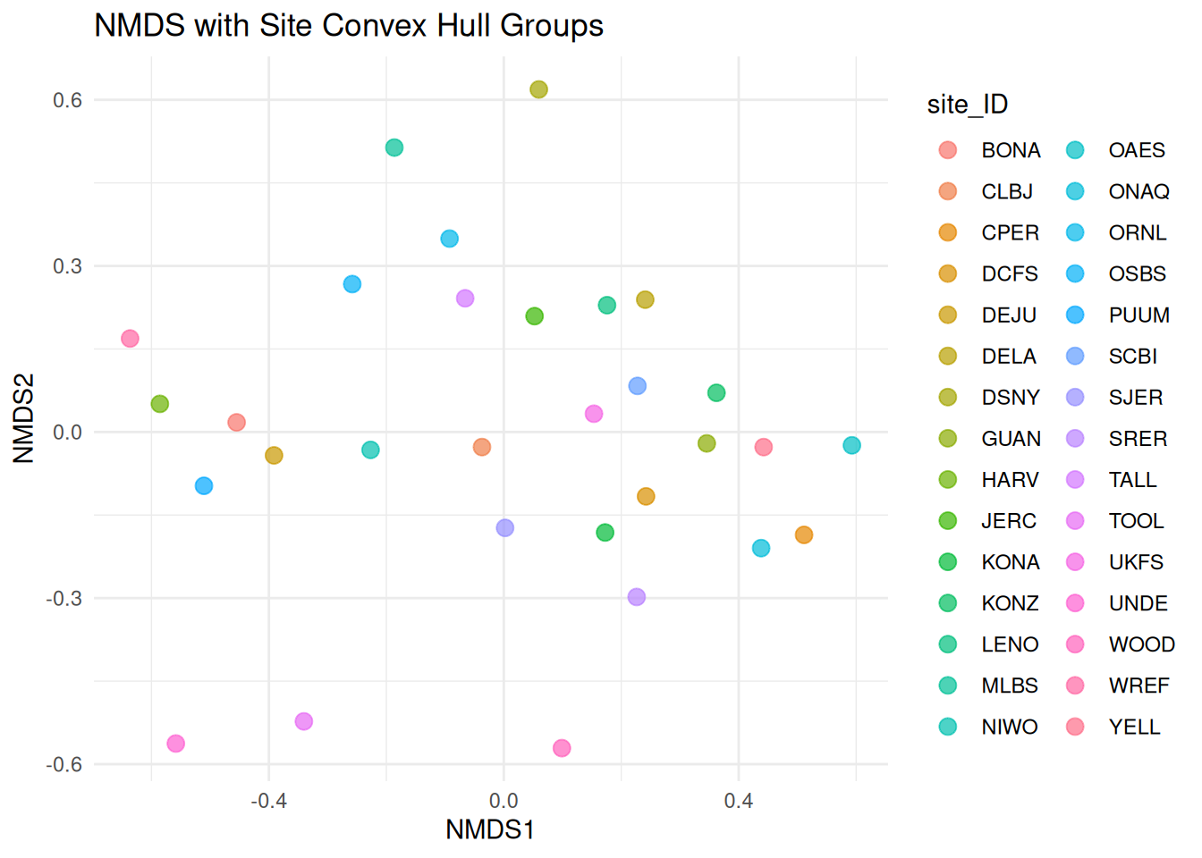
Summary of Observations
Across NEON sites, MAG composition differs at the phylum level.
Shannon diversity and richness values show uneven community structure among locations.
Bray–Curtis clustering and distance heatmaps indicate groups of sites with similar microbial profiles.
PCA and NMDS ordinations both suggest that soil pH and moisture may relate to differences in community composition.
Because read-based abundance data are unavailable, interpretations are based on MAG presence rather than quantitative abundance.